This chapter loads the September 2026 snapshot, checks that it adds up, and then looks at the verdicts one country at a time. The notebook runs top to bottom in a few seconds. Plotting code is folded into a Source bar above each figure; everything else is shown.
from pathlib import Path

import matplotlib.pyplot as plt
import numpy as np
import pandas as pd

import plotstyle
from plotstyle import tidy

REPO = Path("..")  # the CSV sits in the repository root, above book/
VERDICTS = [
    "likely_monetized",
    "possibly_monetized",
    "likely_not_monetized",
    "unable_to_determine",
]

# keep_default_na=False: "NA" is Namibia's code, not a missing value
snapshot = pd.read_csv(
    REPO / "youtube-monetization-signals-by-country.csv", keep_default_na=False
)
snapshot.head()
Three checks come before any analysis: each row’s verdicts add up to its sample size, no published country is under the 30-channel threshold, and the totals match the figures quoted on the other pages of this book.
checked = snapshot["channels_checked"]
assert (snapshot[VERDICTS].sum(axis=1) == checked).all()
assert checked.min() >= 30

countries = len(snapshot)
channels = int(checked.sum())
smallest, largest = int(checked.min()), int(checked.max())
rows_at_60 = int((checked == 60).sum())

# Figures quoted on the text pages of this book
assert (countries, channels) == (50, 3080)
# "one channel in five" could not be determined
assert round(snapshot["unable_to_determine"].sum() / channels, 2) == 0.20
us = snapshot.set_index("country_code").loc["US"]
assert (us["unable_to_determine"], us["channels_checked"]) == (16, 66)

print(f"{countries} countries, {channels:,} channels, "
      f"{smallest} to {largest} per country")
50 countries, 3,080 channels, 54 to 74 per country
All checks pass. The file holds 50 countries and 3,080 channels, with 54 to 74 channels per country; 39 countries have exactly 60.
pooled = snapshot[VERDICTS].sum()
share_text = {
    verdict: f"{pooled[verdict] / channels:.1%}" for verdict in VERDICTS
}
pd.DataFrame(
    {"channels": pooled, "share": [share_text[verdict] for verdict in VERDICTS]}
).rename(index=plotstyle.VERDICT_LABELS)
Loading...
Across all 3,080 channels, 25.5% were rated likely monetized under the September rule, 49.4% possibly monetized, 5.1% likely not monetized, and 20.0% could not be determined.
“Possibly monetized” is the largest group. Part of the reason is the September rule itself. A channel needed a Join button to be rated likely monetized, so a large channel with ads on its videos but no memberships stopped at “possibly”. The last chapter follows that thread.
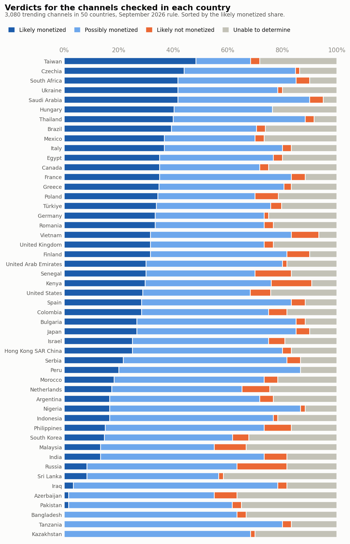
Each bar below is one country, split into the four verdicts. Countries are sorted by the share rated likely monetized.
Source
order = snapshot.assign(likely_share=snapshot["likely_monetized"] / checked).sort_values(
    ["likely_share", "channels_checked"]
)
shares = order[VERDICTS].div(order["channels_checked"], axis=0)

fig, ax = plt.subplots(figsize=(8, 12.5))
left = np.zeros(len(order))
for verdict in VERDICTS:
    ax.barh(
        order["country"],
        shares[verdict],
        left=left,
        height=0.7,
        color=plotstyle.VERDICT_COLOURS[verdict],
        edgecolor=plotstyle.SURFACE,  # thin gap between segments instead of an outline
        linewidth=1.2,
        label=plotstyle.VERDICT_LABELS[verdict],
    )
    left += shares[verdict].to_numpy()

ax.set_xlim(0, 1)
ax.set_ylim(-0.6, len(order) - 0.4)
ax.xaxis.set_major_formatter(plotstyle.PERCENT)
ax.xaxis.set_ticks_position("top")
ax.tick_params(axis="y", labelsize=8.5)
tidy(ax)
ax.spines["bottom"].set_visible(False)
fig.suptitle("Verdicts for the channels checked in each country", x=0.02, ha="left", fontsize=13, fontweight="semibold")
fig.text(
    0.02,
    0.958,
    f"{channels:,} trending channels in {countries} countries, September 2026 rule. Sorted by the likely monetized share.",
    fontsize=9,
    color=plotstyle.INK_SECONDARY,
)
fig.legend(
    loc="upper left",
    bbox_to_anchor=(0.015, 0.948),
    ncol=4,
    frameon=False,
    fontsize=9,
    handlelength=1.2,
    handleheight=1.2,
    columnspacing=1.4,
)
fig.tight_layout(rect=(0, 0, 1, 0.94))
plt.show()
WORDS = "zero one two three four five six seven eight nine ten".split()  # for the text

ranked = order.iloc[::-1]  # highest likely share first
top = ranked.iloc[0]
zeros = ranked.loc[ranked["likely_monetized"] == 0, "country"].tolist()
unable_share = snapshot["unable_to_determine"] / checked
unable_share.index = snapshot["country"]
lowest_unable, highest_unable = unable_share.idxmin(), unable_share.idxmax()
print(f"top: {top['country']} {top['likely_share']:.1%}; none likely: {zeros}")
print(f"unable: {unable_share.min():.1%} ({lowest_unable}) "
      f"to {unable_share.max():.1%} ({highest_unable})")
Taiwan leads at 48.3%. At the other end, three countries had no channel rated likely monetized at all: Bangladesh, Tanzania, Kazakhstan. The grey part of each bar deserves as much attention as the blue. The share we could not call runs from 5.0% in Saudi Arabia to 41.7% in Sri Lanka.
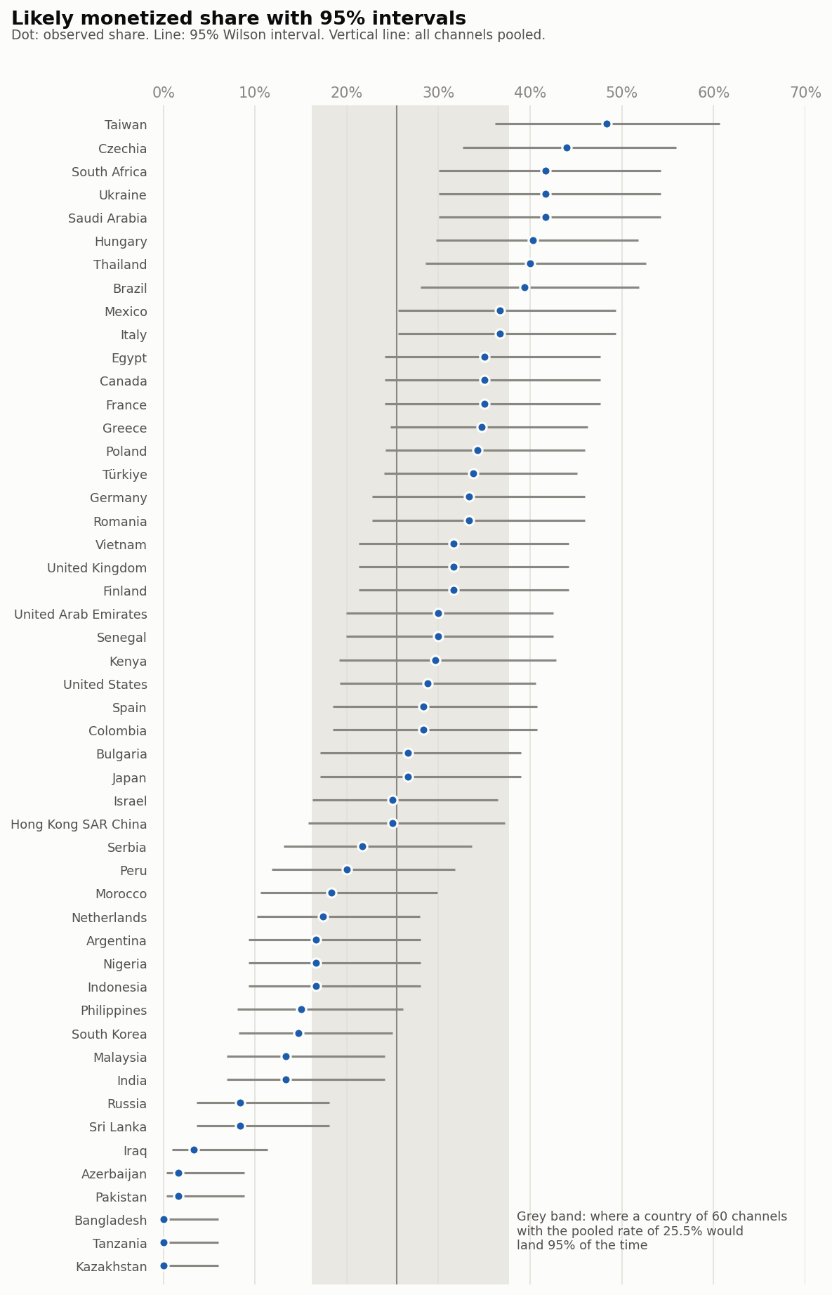
Sixty channels is a small sample for a share. The next cell computes a 95% Wilson interval for each country’s likely monetized share, and the interval a country would have if its true rate were the pooled one.
Z = 1.96  # two-sided 95%


def wilson_interval(hits, n):
    """95% Wilson score interval; stays sensible near 0% and at n of about 60."""
    p = hits / n
    centre = (p + Z**2 / (2 * n)) / (1 + Z**2 / n)
    half_width = Z * np.sqrt(p * (1 - p) / n + Z**2 / (4 * n**2)) / (1 + Z**2 / n)
    return centre - half_width, centre + half_width


pooled_likely = pooled["likely_monetized"] / channels
order["low"], order["high"] = wilson_interval(
    order["likely_monetized"], order["channels_checked"]
)
band_low, band_high = wilson_interval(pooled_likely * 60, 60)

outside = order[(order["low"] > pooled_likely) | (order["high"] < pooled_likely)]
expected_outside = 0.05 * countries

# How far apart two countries of 60 channels each must be, near the pooled
# rate, before a two-proportion z-test at the 5% level calls the gap real
needed_gap = Z * np.sqrt(2 * pooled_likely * (1 - pooled_likely) / 60)
neighbour_gaps = ranked["likely_share"].diff().abs().dropna()

print(f"pooled {pooled_likely:.1%}, n=60 band {band_low:.1%} to {band_high:.1%}")
print(f"{len(outside)} of {countries} intervals leave out the pooled rate, "
      f"about {expected_outside:g} expected by chance")
print(f"gap needed {needed_gap:.1%}, "
      f"median gap between neighbours {neighbour_gaps.median():.1%}")
pooled 25.5%, n=60 band 16.1% to 37.7%
21 of 50 intervals leave out the pooled rate, about 2.5 expected by chance
gap needed 15.6%, median gap between neighbours 0.5%
Source
fig, ax = plt.subplots(figsize=(8, 12.5))
y = np.arange(len(order))
ax.axvspan(band_low, band_high, color=plotstyle.GRID, alpha=0.7, lw=0, zorder=0)
ax.axvline(pooled_likely, color=plotstyle.INK_MUTED, lw=1, zorder=1)
ax.hlines(y, order["low"], order["high"], color=plotstyle.INK_MUTED, lw=1.5, zorder=2)
ax.scatter(
    order["likely_share"], y, s=40, color=plotstyle.VERDICT_COLOURS["likely_monetized"],
    edgecolors=plotstyle.SURFACE, linewidths=1.5, zorder=3,
)
ax.set_yticks(y, order["country"], fontsize=8.5)
ax.set_ylim(-0.8, len(order) - 0.2)
ax.set_xlim(-0.012, 0.7)  # a little room so dots at 0% are not cut
ax.xaxis.set_major_formatter(plotstyle.PERCENT)
ax.xaxis.set_ticks_position("top")
ax.grid(axis="x", color=plotstyle.GRID, lw=0.8)
tidy(ax)
ax.spines["bottom"].set_visible(False)
ax.text(
    band_high + 0.008, 1.5,
    f"Grey band: where a country of 60 channels\nwith the pooled rate of {pooled_likely:.1%} would\nland 95% of the time",
    fontsize=8.5, color=plotstyle.INK_SECONDARY, va="center",
)
fig.suptitle("Likely monetized share with 95% intervals", x=0.02, ha="left", fontsize=13, fontweight="semibold")
fig.text(
    0.02, 0.958,
    "Dot: observed share. Line: 95% Wilson interval. Vertical line: all channels pooled.",
    fontsize=9, color=plotstyle.INK_SECONDARY,
)
fig.tight_layout(rect=(0, 0, 1, 0.96))
plt.show()
A country of 60 channels with the pooled rate of 25.5% could land anywhere from 16.1% to 37.7% by chance alone. Yet 21 of the 50 intervals leave out the pooled rate, where noise alone would leave out about 2.5. So the countries do differ.
What the figure also shows is how little separates neighbours. Near the pooled rate, two countries of 60 channels each have to be about 16 points apart before a two-proportion test at the 5% level calls the gap real. The median gap between neighbouring countries in the ranking is 0.5 points. Reading the order of two adjacent countries as meaningful is reading noise.
The shares so far divide by every checked channel, unknowns included. The next cell recomputes the likely share among the channels we could call, and works out a ceiling: the share a country would reach if every one of its unknowns were in fact monetized.
def rank_correlation(a, b):
    """Spearman's rho: Pearson on average ranks, so no SciPy is needed."""
    return float(np.corrcoef(pd.Series(a).rank(), pd.Series(b).rank())[0, 1])


likely, unknown = order["likely_monetized"], order["unable_to_determine"]
order["share_of_called"] = likely / (order["channels_checked"] - unknown)
order["ceiling"] = (likely + unknown) / order["channels_checked"]
order["unable_share"] = unknown / order["channels_checked"]
rho_called = rank_correlation(order["likely_share"], order["share_of_called"])

columns = {
    "country": "country",
    "channels_checked": "checked",
    "unable_share": "unable",
    "likely_share": "likely, of all checked",
    "share_of_called": "likely, of those called",
    "ceiling": "ceiling",
}
(
    order.nlargest(5, "unable_share")[list(columns)]
    .rename(columns=columns)
    .style.format("{:.1%}", subset=list(columns.values())[2:])
    .hide(axis="index")
)
Loading...
Leaving the unknowns out raises most shares but hardly changes the order: the rank correlation between the two versions is 0.98. The ceiling is a different story. For the five countries with the most unknowns, it sits far above the observed share. Neither extreme is realistic, but the distance between them shows how much a single country’s figure depends on channels we could not read.
medians = snapshot["median_subscribers"]
over_100k = int((medians > 100_000).sum())
# "all but one country" in the introduction, "49 of the 50" in How a verdict is made
assert over_100k == countries - 1 == 49
rho_size = rank_correlation(order["median_subscribers"], order["likely_share"])
print(f"median channel above 100,000 subscribers in {over_100k} countries; "
      f"median of medians {medians.median():,.0f}; "
      f"rank correlation with likely share {rho_size:.2f}")
median channel above 100,000 subscribers in 49 countries; median of medians 397,250; rank correlation with likely share 0.01
These are big channels. In 49 of the 50 countries the median checked channel has more than 100,000 subscribers, and the median across countries is 397,250. If bigger channels simply showed more signals, the ranking would be a ranking of channel size. It is not: across the 50 countries, the rank correlation between median subscribers and the likely monetized share is 0.01.
bottom_eight = ranked.tail(8)
next_share = ranked.iloc[-9]["likely_share"]
next_up = ranked.loc[ranked["likely_share"] == next_share, "country"].tolist()
print(", ".join(bottom_eight["country"]))
print(f"at most {bottom_eight['likely_share'].max():.1%}; "
      f"next up {next_up} at {next_share:.1%}")
Russia, Sri Lanka, Iraq, Azerbaijan, Pakistan, Bangladesh, Tanzania, Kazakhstan
at most 8.3%; next up ['Malaysia', 'India'] at 13.3%
The ranking has a floor. The bottom eight countries (Russia, Sri Lanka, Iraq, Azerbaijan, Pakistan, Bangladesh, Tanzania, Kazakhstan) have at most 8.3% of their channels rated likely monetized; the next countries up, Malaysia and India, have 13.3%. Channel size does not explain that cluster, and neither does sampling noise. The next chapter shows what does.